Stop Scrolling in Excel: Use the Name Box to Jump to Any Cell or Range

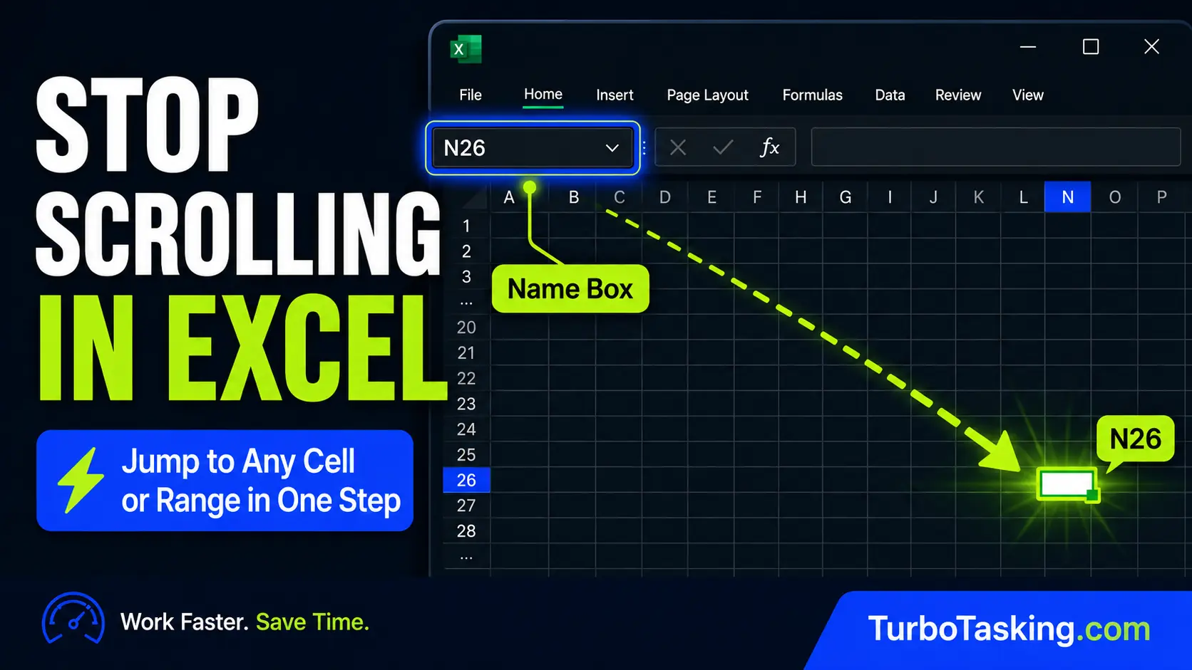
There is a small box in Excel that can save you a surprising amount of scrolling.

It sits above the sheet, just to the left of the formula bar.

Most people only notice it when it shows the current cell address, something like A1, D12, or N26. But that box is not just a label. It is the Excel Name Box, and you can use it to jump to a cell, select a range, and create simple workbook shortcuts for important areas.

If you work with large spreadsheets, this is one of those tiny Excel habits that makes the whole file feel less annoying.

What the Excel Name Box does

The Name Box is the field to the left of the formula bar. Microsoft describes it as a way to quickly locate and select specific cells or ranges by entering their names or cell references. You can type a cell like B3, a range like B1:B3, or select a named cell or range from the dropdown list. Microsoft’s guide to selecting specific cells and ranges explains the same basic workflow.

In plain English, it gives you a direct address bar for your spreadsheet.

Instead of scrolling across columns, dragging through hundreds of rows, or trying to find a tiny section manually, you type where you want to go and press Enter.

• Type N26 to jump to cell N26.
• Type A1:H200 to select that range.
• Select a named range like PricingTable from the dropdown.
• Create a name for the current selection by typing a name in the Name Box and pressing Enter.

That last point is the one many Excel users miss. You do not always need to open Name Manager or use a ribbon command just to create a simple named range.

The fastest way to jump to a cell

Imagine someone asks you to check cell N26.

The slow way is to scroll right, scroll down, overshoot the row, move back, then click the cell.

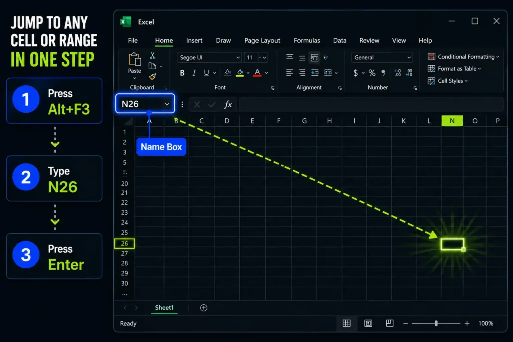
The faster way is:

1. Put the cursor in the Name Box.
2. Type N26.
3. Press Enter.

Excel jumps straight to that cell.

On my Excel for Windows setup, Alt + F3 puts the focus directly in the Name Box. That makes the workflow very fast:

Alt + F3, type N26, press Enter.

If Alt + F3 does not work in your version of Excel, use the Go To dialog instead. Press F5 or Ctrl + G, type the cell reference, and press Enter. Microsoft lists F5 and Ctrl + G as shortcuts for the Go To dialog in its Excel keyboard shortcuts documentation.

Use the Name Box to select a range without dragging

The Name Box is not only for single cells. It can also select a range by address.

For example, you can type:

• A1:A500 to select one long column range.
• A1:H200 to select a rectangular data area.
• D10:F20 to select a smaller block in the middle of a sheet.

This is useful when you already know the range you need, especially in large files where dragging is slow and error-prone.

Typical office examples:

• Select a monthly data area before applying formatting.
• Select a long list before copying it to another workbook.
• Select an input range before clearing old values.
• Select a report block before adding borders or number formatting.
• Select a lookup table before converting it into a table.

This is also safer than dragging when the range is larger than your screen. If you type A1:H500, Excel selects exactly that range. It does not depend on how steady your mouse hand is.

Turn important cells into workbook bookmarks

The real productivity gain starts when you stop treating named ranges as an “Excel formula feature” and start treating them as bookmarks inside your workbook.

For example, instead of remembering that your exchange rate is in Inputs!F12, you can name that cell ExchangeRate.

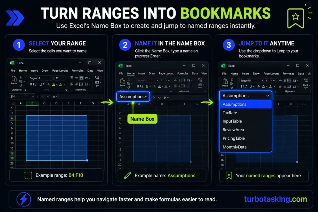
Instead of remembering that your assumptions area is B4:F18, you can name it Assumptions.

Then you can jump back to those areas from the Name Box dropdown or by typing the name directly.

How to create a named range from the Name Box

1. Select the cell or range you want to name.
2. Click the Name Box, or press Alt + F3 if it works in your Excel.
3. Type a name, for example TaxRate, InputTable, or ReviewArea.
4. Press Enter.

Microsoft’s documentation also shows that you can name a cell by selecting it, typing a name in the Name Box, and pressing Enter. The same documentation explains how names can be used in formulas and managed later from Name Manager. See Microsoft’s guide to defining and using names in formulas.

One important detail: after typing the name, press Enter. If you type the name and then click somewhere else, Excel may not create the name.

Name Box vs Go To: they are connected

The Name Box and Go To are closely related.

Both can take you to a cell reference. Both can take you to a named range. Both can select a range by address.

The difference is how you access them.

Use this	When it is best	Example
Name Box	When you want a fast address bar above the sheet	Type N26 or A1:H200
Name Box dropdown	When you have named ranges and want to jump visually	Select Assumptions
Go To, F5 or Ctrl + G	When you want a keyboard-friendly dialog	Type B3, B1:B3, or a named range
Go To Special	When you want to select cells by condition	Blanks, formulas, constants, visible cells only

For everyday navigation, I prefer the Name Box because it is simple and visible. For more advanced selection tasks, Go To Special is often better.

Use Name Manager when the workbook needs cleanup

The Name Box is great for creating and using simple names. But it is not where you edit or delete them.

For that, use Name Manager.

Go to Formulas > Name Manager, or use Ctrl + F3.

Name Manager is where you can review names, edit references, delete old names, and check whether the workbook contains confusing or broken named ranges. Microsoft describes it as the central place to create, edit, delete, and filter names in an Excel workbook. See Microsoft’s Name Manager guide.

This matters in shared office files. A workbook can collect old names over time, especially if people copy sheets from other files. If the Name Box dropdown is full of unclear names, Name Manager is where you clean that up.

Use Create from Selection when labels already exist

There is another useful named range feature: Create from Selection.

This is useful when your worksheet already has labels in the top row or left column, and you want Excel to create names from those labels.

For example, suppose you have a small assumptions table like this:

Input	Value
TaxRate	19%
DiscountRate	5%
ExchangeRate	1.08

You can select the table and use Formulas > Defined Names > Create from Selection. The shortcut is Ctrl + Shift + F3. Microsoft also lists this workflow in its guide to creating a named range from selected cells.

I would not use this everywhere. But it is handy when you have clean labels and want to turn them into usable names quickly.

Use names to make formulas easier to read

Named ranges are not only useful for navigation. They can also make formulas easier to understand.

Compare this:

=B12*$F$3

With this:

=B12*TaxRate

The second formula tells you what the reference means. You do not need to remember what is stored in $F$3.

This is especially helpful for small input cells used across a workbook:

• TaxRate
• ExchangeRate
• StartDate
• EndDate
• DiscountRate
• TargetMargin

Do not overdo it. A few meaningful names can make a workbook clearer. Dozens of vague names can make it harder to audit.

Go To Special: the advanced version of “jump and select”

Once you are comfortable with F5 or Ctrl + G, the next useful feature is Go To Special.

Open Go To, then choose Special. Excel can select cells that match specific conditions, such as formulas, constants, blanks, objects, visible cells only, or the last cell used in the worksheet.

That sounds technical, but it is very practical in office work.

• Select blanks before filling missing values.
• Select formulas before checking what is calculated and what is manually typed.
• Select constants before identifying hardcoded numbers.
• Select visible cells only before copying filtered data.
• Select the last used cell to diagnose a worksheet that behaves as if it has thousands of extra rows.

Microsoft mentions Go To Special as a way to quickly find and select cells that contain specific types of data, such as formulas, visible cells only, or the last cell on the worksheet that contains data or formatting. See the Go To section in Microsoft’s guide.

The Excel navigation shortcuts I would learn with the Name Box

The Name Box is useful on its own, but it becomes better when you combine it with a few keyboard shortcuts.

You do not need to memorize every Excel shortcut. These are the ones that fit the same job: move faster through a workbook and select the right area without dragging.

Shortcut	What it does	When to use it
Alt + F3	Moves focus to the Name Box on my Excel for Windows setup	Jump to a cell or type a range without clicking
F5	Opens Go To	Jump to a cell, range, or named range
Ctrl + G	Opens Go To	Same as F5, useful if your keyboard makes F-keys awkward
Ctrl + F3	Opens Name Manager	Edit, delete, or review named ranges
Ctrl + Shift + F3	Creates names from selected labels	Turn labeled rows or columns into names
F3	Opens Paste Name when names exist	Insert a named range into a formula
Ctrl + Arrow	Moves to the edge of the current data region	Move across a table quickly
Ctrl + Shift + Arrow	Extends the selection to the last nonblank cell	Select data without dragging
Ctrl + Home	Moves to the beginning of the worksheet	Return to the top-left area quickly
Ctrl + End	Moves to the last used cell	Check where Excel thinks the sheet ends
Ctrl + Space	Selects the current column	Format or inspect a whole column
Shift + Space	Selects the current row	Format or inspect a whole row

Several of these shortcuts are listed in Microsoft’s official Excel keyboard shortcuts page.

A simple workflow for large office spreadsheets

Here is how I would use this in a real office workbook.

When you receive or create a workbook that you will use repeatedly, spend two minutes naming the parts you will revisit.

1. Select the main input area and name it Inputs.
2. Select the assumptions block and name it Assumptions.
3. Select the final report area and name it Output.
4. Select important single cells and give them clear names, such as TaxRate or StartDate.
5. Use the Name Box dropdown to jump between those areas later.

This gives you a lightweight navigation system inside the workbook.

It is especially useful for files that you open every week or every month:

• Monthly reporting templates.
• Budget files.
• Forecast models.
• Project trackers.
• Invoice lists.
• Data cleanup workbooks.
• Shared team templates.

You are not just making formulas cleaner. You are making the workbook easier to navigate.

Good names vs bad names

A named range is only useful if the name is clear.

Use names that explain the purpose of the cell or range.

Better	Worse
TaxRate	Rate1
StartDate	DateA
InputTable	Range1
Assumptions	Block
FinalReport	Area2

Keep names short, but not cryptic.

I also prefer names without spaces. Excel names cannot behave like normal sentences, so use a readable format like TaxRate, Tax_Rate, or monthly_sales. Pick one style and stay consistent.

Common mistakes to avoid

1. Typing a name but not pressing Enter

When you create a name from the Name Box, press Enter. Otherwise, you may think you created a name, but nothing was saved.

2. Creating too many names

Do not name every small area of a workbook. Name the parts you need to revisit, explain, audit, or reuse in formulas.

3. Using vague names

Range1 is not much better than B4:F18. If the name does not explain what the range means, it will not help much.

4. Forgetting Name Manager exists

The Name Box is fast for creating and using names, but Name Manager is where you review, edit, and delete them.

5. Using named ranges when an Excel table would be better

If your data grows every week, an Excel table may be better than a fixed named range. Named ranges are great for inputs, assumptions, fixed areas, and navigation bookmarks. For expanding datasets, use Excel tables when possible.

When I would use the Name Box

I would use the Name Box when the problem is navigation or precise selection.

• You know the cell address and want to get there instantly.
• You need to select a large range without dragging.
• You revisit the same areas of a workbook repeatedly.
• You want formulas to use names like TaxRate instead of raw references like $F$3.
• You are building a workbook that someone else will need to understand.

I would not turn every workbook into a named range system. For a quick one-off spreadsheet, it may not be worth it.

But for recurring workbooks, shared templates, reports, and large sheets, the Name Box is worth learning.

Stop treating the Name Box as decoration

The Excel Name Box looks like a small detail, but it changes how you move through large spreadsheets.

At the basic level, it is a jump box: type N26 and go there.

At the next level, it is a range selector: type A1:H500 and select exactly that block.

At the most useful level, it is a simple bookmark system for your workbook: name the areas that matter and stop hunting for them manually.

Learn the Name Box, F5, Ctrl + G, Ctrl + F3, and a few navigation shortcuts. You will spend less time scrolling and more time actually working with the spreadsheet.